There have been some exciting developments in the Deducer ecosystem over the summer which should go into CRAN release in the next few months. Today I’m going to give a quick sneak peek at an Open Street Map – R connection with accompanying GUI. This post will just show the non-GUI components.
The first part of the project was to create a way to download and plot Open Street Map data from either Mapnik or Bing in a local R instance. Before we can do that however, we need to install DeducerSpatial.
install.packages(c("Deducer","sp","rgdal","maptools"))
install.packages("UScensus2000")

#get development versions
install.packages(c("JGR","Deducer"),,"http://rforge.net",type="source")
install.packages("DeducerSpatial",,"http://r-forge.r-project.org",type="source")
Note that you will need rgdal. And you will need your development tools to install the development versions of JGR, Deducer and DeducerSpatial.
Plot an Open Street Map Image
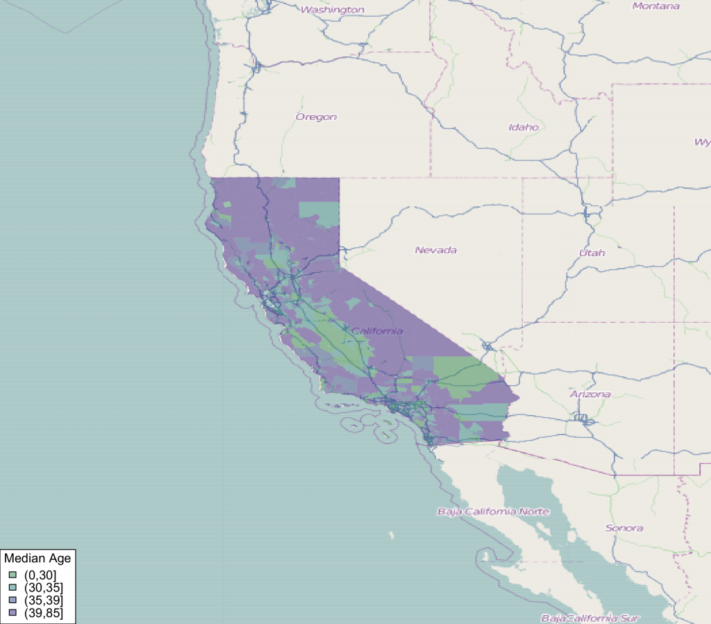
We are going to take a look at the median age of households in the 2000 california census survey. First, lets see if we can get the open street map image for that area.
#load package
library(DeducerSpatial)
library(UScensus2000)

#create an open street map image
lat <- c(43.834526782236814,30.334953881988564)
lon <- c(-131.0888671875  ,-107.8857421875)
southwest <- openmap(c(lat[1],lon[1]),c(lat[2],lon[2]),zoom=5,'osm')
plot(southwest,raster=FALSE)
Note that plot has an argument ‘raster’ which determines if the image is plotted as a raster image. ‘zoom’ controls the level of detail in the image. Some care needs to be taken in choosing the right level of zoom, as you can end up trying to pull street level images for the entire world if you are not careful.
Make a Choropleth Plot
Next, we can add a choropleth to the plot. We bring in the census data from the UScensus2000 package, and transform it to the mercator projection using spTransform.
#load in califonia data and transform coordinates to mercator
data(california.tract)
california.tract <- spTransform(california.tract,osm())

#add median age choropleth
choro_plot(california.tract,dem = california.tract@data[,'med.age'],
	legend.title = 'Median Age')
Use Aerial Imagery
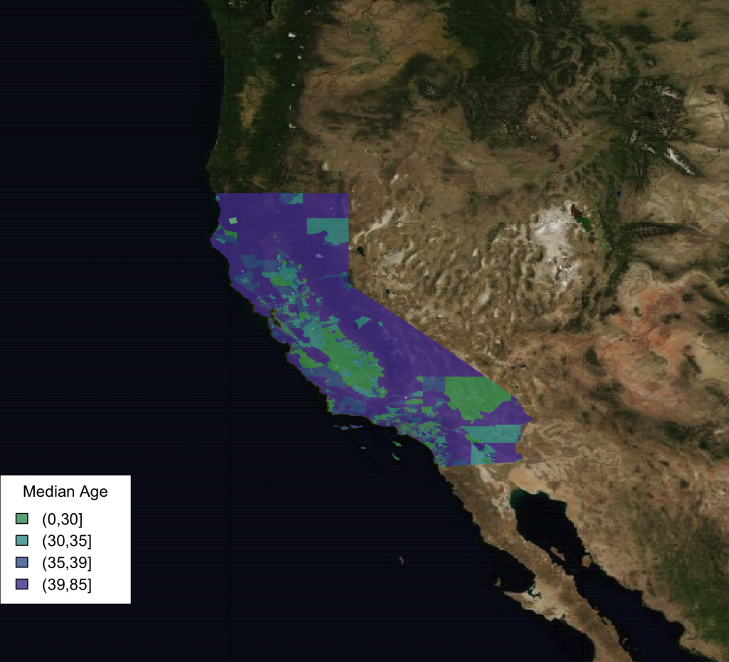
We can also easily use bing satellite imagery instead.
southwest <- openmap(c(lat[1],lon[1]),c(lat[2],lon[2]),5,'bing')
plot(southwest,raster=FALSE)
choro_plot(california.tract,dem = california.tract@data[,'med.age'],alpha=.8,
	legend.title = 'Median Age')
One other fun thing to note is that the image tiles are cached so they do not always need to be re-downloaded.
> system.time(southwest <- openmap(c(lat[1],lon[1]),c(lat[2],lon[2]),zoom=7,'bing'))
   user  system elapsed
  9.502   0.547  17.166
> system.time(southwest <- openmap(c(lat[1],lon[1]),c(lat[2],lon[2]),zoom=7,'bing'))
   user  system elapsed
  9.030   0.463   9.169
Notice how the elapsed time in the second call is half that of the first one, this is due to caching.
This just scratches the surface of what is possible with the new package. You can plot any type of spatial data (points, lines, etc.) supported by the sp package so long as it is in the mercator projection. Also, there is a full featured GUI to help you load your data and make plots, but I’ll talk about that in a later post.


2 replies on “Open Street maps”
You should note that anyone having troubles installing the dev versions should include:
Sys.setenv(NOAWT=1)
prior to the install.packages() commands.
Nice post otherwise!
Thanks, that is required on the Mac. Also, Deducer (and DeducerSpatial) must be run through JGR on OS X.