Category: Spatial

A new version of the OpenStreetMap package has been released to CRAN. OpenStreetMap 0.3.3 contains several minor improvements. I’ve removed the CloudMade tile set types, as they seem to have gone out of business. MapQuest has also been removed as they have moved to a new API. The mapbox type has been updated to use their new API.

The most important update is the ability to use custom tile servers. Suppose you have a server using the tile map service specification with access urls looking something like

http://api.someplace.com/{z}/{x}/{y}.png*

where {z} is the map’s integer zoom level, {x} is the tile’s integer x position and {y} is the tile’s integer y position. You may pass this url into openmap’s type argument to obtain a map using this tileset.

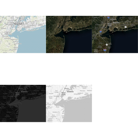
For example, if you need to access MapQuest’s tilesets, which now require a developer API key, you can use the new custom tileserver facility to access them. Below is an example with my (free) API key.

 

ul <- c(40.9,-74.5)
lr <- c(40.1,-73.2)
par(mfrow=c(2,3))
url <- "https://a.tiles.mapbox.com/v4/mapquest.streets-mb/{z}/{x}/{y}.png?access_token=pk.eyJ1IjoibWFwcXVlc3QiLCJhIjoiY2Q2N2RlMmNhY2NiZTRkMzlmZjJmZDk0NWU0ZGJlNTMifQ.mPRiEubbajc6a5y9ISgydg"
map <- openmap(ul,lr,minNumTiles=4, type=url)
plot(map)


url <- "https://a.tiles.mapbox.com/v4/mapquest.satellitenolabels/{z}/{x}/{y}.png?access_token=pk.eyJ1IjoibWFwcXVlc3QiLCJhIjoiY2Q2N2RlMmNhY2NiZTRkMzlmZjJmZDk0NWU0ZGJlNTMifQ.mPRiEubbajc6a5y9ISgydg"
map <- openmap(ul,lr,minNumTiles=4, type=url)
plot(map)


url <- "https://a.tiles.mapbox.com/v4/mapquest.satellite/{z}/{x}/{y}.png?access_token=pk.eyJ1IjoibWFwcXVlc3QiLCJhIjoiY2Q2N2RlMmNhY2NiZTRkMzlmZjJmZDk0NWU0ZGJlNTMifQ.mPRiEubbajc6a5y9ISgydg"
map <- openmap(ul,lr,minNumTiles=4, type=url)
plot(map)

url <- "https://a.tiles.mapbox.com/v4/mapquest.dark/{z}/{x}/{y}.png?access_token=pk.eyJ1IjoibWFwcXVlc3QiLCJhIjoiY2Q2N2RlMmNhY2NiZTRkMzlmZjJmZDk0NWU0ZGJlNTMifQ.mPRiEubbajc6a5y9ISgydg"
map <- openmap(ul,lr,minNumTiles=4, type=url)
plot(map)

url <- "https://a.tiles.mapbox.com/v4/mapquest.light/{z}/{x}/{y}.png?access_token=pk.eyJ1IjoibWFwcXVlc3QiLCJhIjoiY2Q2N2RlMmNhY2NiZTRkMzlmZjJmZDk0NWU0ZGJlNTMifQ.mPRiEubbajc6a5y9ISgydg"
map <- openmap(ul,lr,minNumTiles=4, type=url)
plot(map)

 

 

 

 

 

A new version of the OpenStreetMap package is now up on CRAN, and should propagate to all the mirrors in the next few days. The primary purpose of the package is to provide high resolution map/satellite imagery for use in your R plots. The package supports base graphics and ggplot2, as well as transformations between spatial coordinate systems.

The bigest change in the new version is the addition of dozens of tile servers, giving the user the option of many different map looks, including those from Bing, MapQuest and Apple.

nm = c("osm", "maptoolkit-topo",
"waze", "mapquest", "mapquest-aerial",
"bing", "stamen-toner", "stamen-terrain",
"stamen-watercolor", "osm-german", "osm-wanderreitkarte",
"mapbox", "esri", "esri-topo",
"nps", "apple-iphoto", "skobbler",
 "opencyclemap", "osm-transport",
"osm-public-transport", "osm-bbike", "osm-bbike-german")

png(width=1200,height=2200)
par(mfrow=c(6,4))
for(i in 1:length(nm)){
	print(nm[i])
	map = openmap(c(lat= 38.05025395161289,   lon= -123.03314208984375),
			c(lat= 36.36822190085111,   lon= -120.69580078125),
			minNumTiles=9,type=nm[i])
	plot(map)
	title(nm[i],cex.main=4)
}
dev.off()

You can also render maps from cloudmade.com which hosts tons of map tilings. Simply set the “type” parameter to “cloudmade-<id>” where <id> is the cloudmade identifier for the map you want to use. Here is a sample:

nm = c("cloudmade-2","cloudmade-999","cloudmade-998",
"cloudmade-7","cloudmade-1960","cloudmade-1155",
"cloudmade-12284")
#setCloudMadeKey("<your key>")
png("RPlot002.png",width=1300,height=800)
par(mfrow=c(2,4))
for(i in 1:length(nm)){
	print(nm[i])
	map = openmap(c(lat= 38.05025395161289,   lon= -123.03314208984375),
			c(lat= 36.36822190085111,   lon= -120.69580078125),
			minNumTiles=9,type=nm[i])
	plot(map)
	title(nm[i],cex.main=4)
}
dev.off()

Maps are initially put in a sperical mercator projection which is the standard for most (all?) map tiling systems, but can easily be translated to long-lat (or any other projection) using the openproj function. Maps can be plotted in ggplot2 using the autoplot function.

mapLatLon = openproj(map)
autoplot(mapLatLon)

The package also has a Java GUI to help with map type selection, and specification of coordinates to bound your map. clicking on the map will give you the latitude and longitude of the point clicked.

launchMapHelper()

Probably the main alternative to OpenStreetMap is the ggmap package. ggmap is an excellent package, and it is somewhat unfortunate that there is a significant duplication of effort between it and OpenStreetMap. That said, there are some differences that may help you decide which to use:

Reasons to favor OpenStreetMap:

• More maps: OpenStreetMap supports more map types.
• Better image resolution: ggmap only fetches one png from the server, and thus is limited to the resolution of that png, whereas OpenStreetMap can download many map tiles and stich them together to get an arbitrarily high image resolution.
• Transformations: OpenStreetMap can be used with any map coordinate system, whereas ggmap is limited to long-lat.
• Base graphics: Both packages support ggplot2, but OpenStreetMap also supports base graphics.

 

 

 

A new package OpenStreetMap has been released to CRAN this week which is designed to allow you to easily add satellite imagery, or open street maps to your plots. Raster maps are a great way to add context to your spatial data with a minimum outlay of effort.

The syntax in OpenStreetMap is fairly simple, just give it a bounding box in lat/long and it will download a high quality raster image ready for plotting


library(OpenStreetMap)
library(rgdal)
map plot(map)

(click for higher quality image)

The above code downloads multiple map tiles and stitches together, with the level of zoom determined automatically. Unlike RGoogleMaps no files are created or stored on the hard drive. The plot gets is images from the mapnik server, which can provide street level information. In my opinion, there rendering looks pretty clean as well.

We can also access satellite imagery though Bing.


map plot(map)

Now, that is all fine and dandy, but kind of useless unless you are able to combine it with your own data. Open street map, and Bing (and Google maps) use a particular form of the Mercator projection which has the properties that angles are preserved, and tiles on multiple zoom levels can be stitched together. You can access this projection with the ‘osm’ function.

In terms of combining maps with your data there are two options. The data can be transformed to the osm() projection, or the raster map can be translated to whatever projection the data are in. Here is an example of the first option:

library(UScensus2000)
data(california.tract)
lat lon southwest california.tract plot(southwest)
plot(california.tract,add=TRUE,col=(california.tract@data$med.age>40)+4)


Here we take a map from the UScensus2000 package, transform it to mercator coordinates, and make a choropleth. The spTransform function is a great easy way to project your data into different map coordinate systems.

We may also want to go the other way and transform the image. The openproj function can transform open street maps to different projections. Here is an example combining OpenStreetMap with the maps library by projecting the map into longlat coordinates.

map map_longlat plot(map_longlat,raster=TRUE)
map("world",col="red",add=TRUE)

but, we are not just limited to the longlat projection, we can also do weirder ones like the lambert conic conformal.

map c(40,179),zoom=2,type='bing')
map_longlat #Lambert Conic Conformal (takes some time...)
map_llc "+proj=lcc +lat_1=33 +lat_2=45 +lat_0=39 +lon_0=-96")
plot(map_llc,raster=TRUE)
#add choropleth
data(states)
st_llc plot(st_llc,add=T,col=heat.colors(48,.4)[slot(st_llc,"data")[["ORDER_ADM"]]])


Now, I have no idea why you would want to use this projection, but it is pretty cool none the less.

One of the best uses for raster maps is in street level data, where it is particularly important to give the reader contextual information. Here is a plot of some locations in the Long Beach harbor, using the LA_places dataset.

data(LA_places)
xy map c(33.73290566922855,-118.17521095275879))
png(width = 1000, height = 1000)
plot(map,raster=TRUE)
plot(LA_places,add=TRUE,col="red")
text(xy[,1],xy[,2],slot(LA_places,"data")[,'NAME'],adj=1)

If you are a Deducer user, the DeducerSpatial package provides a GUI for spatial plotting using the OpenStreetMap package.