So as a follow-up to the last post about the 2010-11 state of the union addresses, I was going to compare the 2011 to the new 2012 speech. It looks like Simply Statistics beat me to it, which is very gratifying. No need to do the work myself 🙂
Month: January 2012
The word cloud is a commonly used plot to visualize a speech or set of documents in a succinct way. I really like them. They can be extremely visually pleasing, and you can spend a lot of time perusing over the words gaining new insights.
That said, they don’t convey a great deal of information. From a statistical perspective, a word cloud is equivalent to a bar chart of univariate frequencies, but makes it more difficult for the viewer to estimate the relative frequency of two words. For example, here is a bar chart and word cloud of the state of the union address for 2010 and 2011 combined.
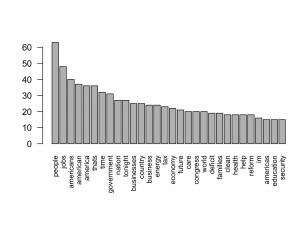
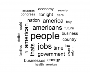
Notice that the bar chart contains more information, with the exact frequencies being obtainable by looking at the y axis. Also, in the word cloud the size of the word both represents the frequency, and the number of characters in the word (with longer words being bigger in the plot). This could lead to confusion for the viewer. We can therefore see that from a statistical perspective that the bar chart is superior.
… Except it isn’t ….
The word cloud looks better. There is a reason why every infographic on the web uses word clouds. It’s because they strike a balance of presenting the quantitative information, while keeping the reader interested with good design. Below I am going to present some extensions of the basic word cloud that help visualize the differences and commonalities between documents.
The Comparison Cloud
The previous plots both pooled the two speeches together. Using standard word clouds that is as far as we can go. What if we want to compare the speeches? Did they talk about different things? If so, are certain words associated with those subjects?
This is where the comparison cloud comes in.
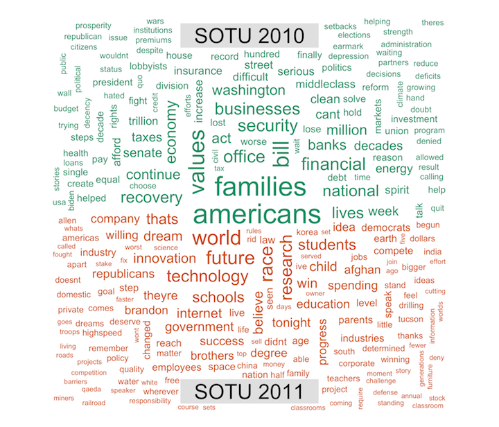
Word size is mapped to the difference between the rates that it occurs in each document. So we see that Obama was much more concerned with economic issues in 2010, and in 2011 focused more on education and the future. This can be generalized fairly naturally. The next figure shows a comparison cloud for the republican primary debate in new hampshire.
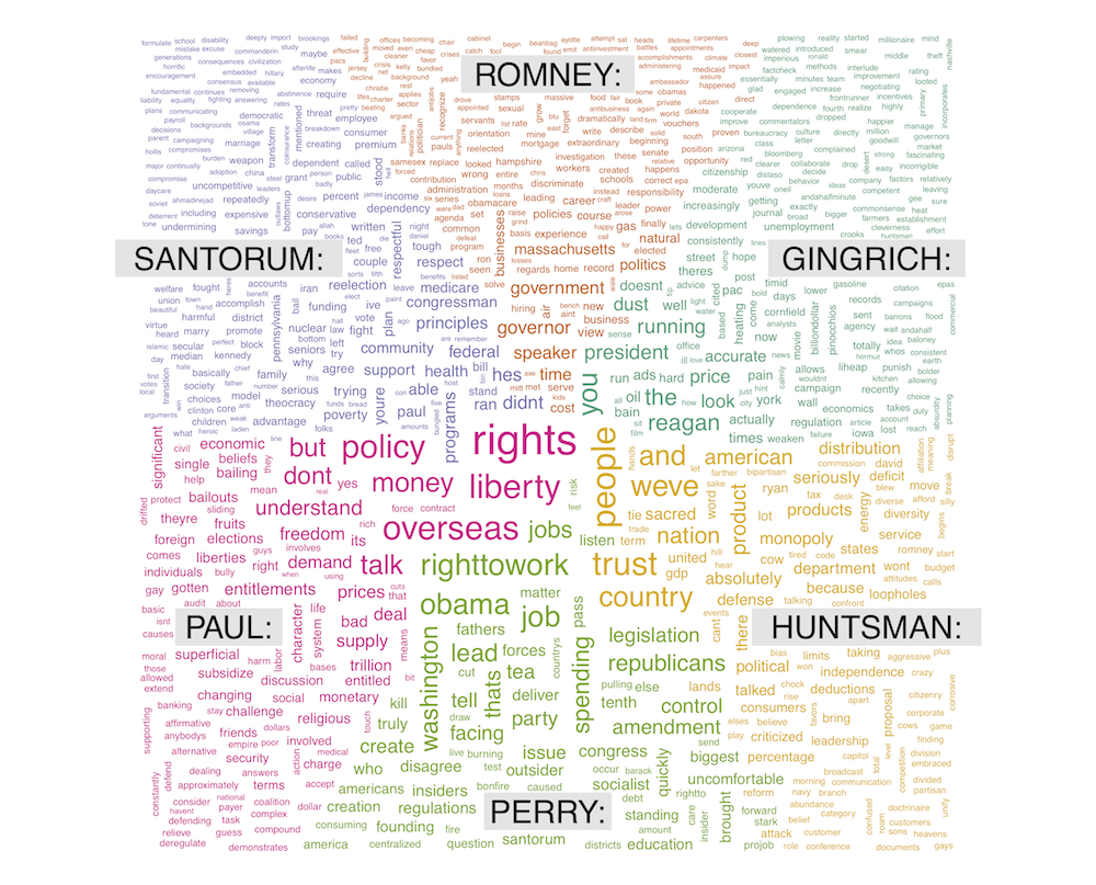 One thing that you can notice in this plot is that Paul, Perry and Huntsman have larger words than the top tier candidates, meaning that they deviate from them mean frequencies more. On the one hand this may be due to a single minded focus on a few differentiating issues (..couch.. Ron Paul), but it may also reflect that the top tier candidates were asked more questions and thus focused on a more diverse set of issues.
The Commonality Cloud
Where the comparison cloud highlights differences, the commonality cloud highlights words common to all documents/speakers. Here is one for the two state of the union addresses.
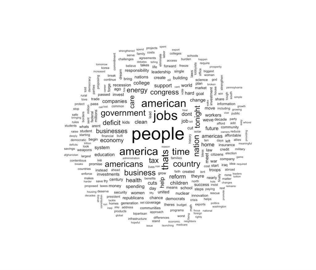
Here, word size is mapped to its minimum frequency across documents. So if a word is missing from any document it has size=0 (i.e. it is not shown). We can also do this on the primary debate data…
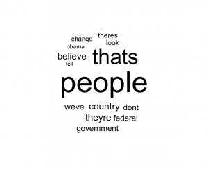
From this we can infer that what politicians like more than anything else is people 🙂
The wordcloud package
Version 2.0 of wordcloud (just released to CRAN) implements these two types of graphs, and the code below reproduces them.
library(wordcloud)
library(tm)
data(SOTU)
corp <- SOTU
corp <- tm_map(corp, removePunctuation)
corp <- tm_map(corp, removePunctuation)
corp <- tm_map(corp, tolower)
corp <- tm_map(corp, removeNumbers)
corp <- tm_map(corp, function(x)removeWords(x,stopwords()))

term.matrix <- TermDocumentMatrix(corp)
term.matrix <- as.matrix(term.matrix)
colnames(term.matrix) <- c("SOTU 2010","SOTU 2011")
comparison.cloud(term.matrix,max.words=300,random.order=FALSE)
commonality.cloud(term.matrix,random.order=FALSE)

library(tm)
library(wordcloud)
library(stringr)
library(RColorBrewer)
repub <- paste(readLines("repub_debate.txt"),collapse="\n")
r2 <- strsplit(repub,"GREGORY\\:")[[1]]
splitat <- str_locate_all(repub,
	"(PAUL|HILLER|DISTASOS|PERRY|HUNTSMAN|GINGRICH|SANTORUM|ROMNEY|ANNOUNCER|GREGORY)\\:")[[1]]
speaker <- str_sub(repub,splitat[,1],splitat[,2])
content <- str_sub(repub,splitat[,2]+1,c(splitat[-1,1]-1,nchar(repub)))
names(content) <- speaker
tmp <- list()
for(sp in c("GINGRICH:"  ,"ROMNEY:"  ,  "SANTORUM:","PAUL:" ,     "PERRY:",     "HUNTSMAN:")){
	tmp[sp] <- paste(content[sp==speaker],collapse="\n")
}
collected <- unlist(tmp)

rcorp <- Corpus(VectorSource(collected))
rcorp <- tm_map(rcorp, removePunctuation)
rcorp <- tm_map(rcorp, removeNumbers)
rcorp <- tm_map(rcorp, stripWhitespace)
rcorp <- tm_map(rcorp, tolower)
rcorp <- tm_map(rcorp, function(x)removeWords(x,stopwords()))
rterms <- TermDocumentMatrix(rcorp)
rterms <- as.matrix(rterms)
comparison.cloud(rterms,max.words=Inf,random.order=FALSE)
commonality.cloud(rterms)
Link to republican debate transcript