Fells Stats

SARS-Cov-2 (COVID-19) has been the defining driver of the market since its emergence. Understanding the progression of the disease through the world has been the secret sauce of alpha generation. Correctly parsing the early infectivity and morality data allowed some to avoid the COVID crash and a solid reading into phase II and phase III vaccine readouts in fall gave insight into the rebound.

As the novel coronavirus raged through the world infecting 181 million and killing 3.9 million (that we know about), the number of people with natural resistance, due to a previous SARS-Cov-2 infection rose. When the virus comes into contact with someone with a resistance, this creates an evolutionary pressure to evade that resistance and re-infect them. Viruses mutate the most when there are high infection rates and lots of people with resistance to it.

It should be no surprise then that more infective variants start to pop up over time, out competing the original strain in the virus’s single-minded goal of using all of us as incubators for self-reproduction. One particular variant of concern is the so-called Delta variant. In this article I’m going to take a look at where we stand with the Delta variant and take a stab at outlining what I view as the most likely trajectory moving forward.

The Delta Variant

The Delta variant emerged in India and is spreading rapidly on a global scale. There currently isn’t strong evidence that it has a much higher mortality rate compared to the original strain, which has a case fatality rate 10-40 times higher than seasonal influenza. Preliminary findings from England and Scotland point to hospitalization rates over 2 times higher than the original strain, so as more studies are performed it would not be surprising to find out that it has increased mortality.

Delta does appear to be much more infectious. Infectiousness can be measured a number of ways. One of these is the relative speed with which it becomes the dominant strain once it enters a population.

Source: Campbell, Finlay, et al. “Increased transmissibility and global spread of SARS-CoV-2 variants of concern as at June 2021.” Eurosurveillance 26.24 (2021): 2100509.

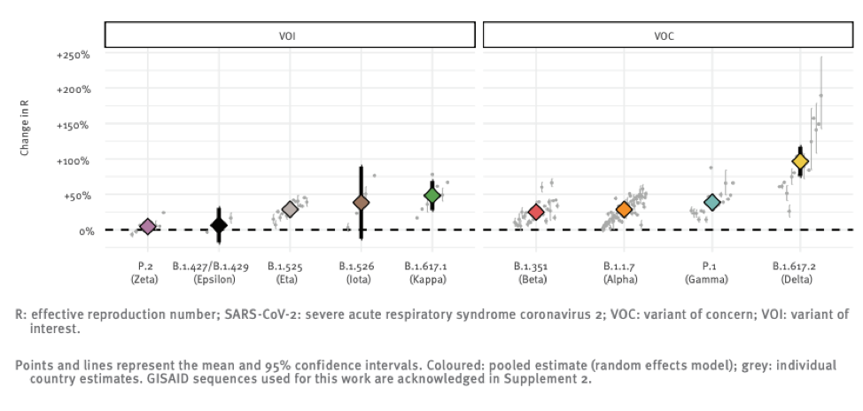
The above chart shows the reproductive number (i.e. the number of people each infected individual infects) relative to the original strain of a number of variants that the global public health community is monitoring. You can see that Delta really breaks away from the pack in terms of infectiousness with a ~100% increase over “regular” SARS-CoV-2.

The original strain is roughly 2 times more infectious than the flu, so this new strain might be 4 times more infectious than seasonal flu. It is hard to overstate just how big a difference this is. The mitigation measures the world put into place in 2020 essentially eradicated seasonal influenza, and yet we still experienced wave after wave of Covid cases.

Where Is It?

The chart below shows the relative prevalence of each of the strains across a number of counties. It is an updated version of one shown in the linked paper that includes additional data collected over the last three weeks, which the authors have graciously allowed me to share.

Source: Campbell, Finlay, et al. “Increased transmissibility and global spread of SARS-CoV-2 variants of concern as at June 2021.” Eurosurveillance 26.24 (2021): 2100509.

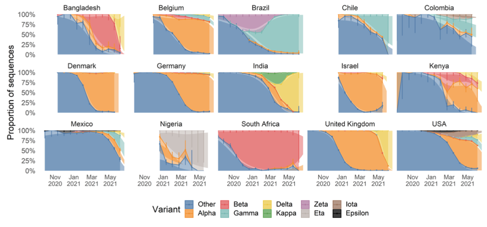
As we can see, Delta first broke out in India and spread to Bangladesh and the UK where it quickly became responsible for the bulk of infections.  Other countries are now seeing spread, with roughly 20% of US infections now being attributable to Delta.

India and Bangladesh both have very young populations, which affords some protection against the ravages of Covid, since the elderly experience the worst outcomes. Unfortunately, this demographic protection was not enough to avoid poor outcomes.

India experienced a well-documented outbreak that severely impacted the country’s people and economy.

Source: https://91-divoc.com/pages/covid-visualization/

Bangladesh is still in the exponential growth phase of the Delta variant. We don’t yet know when it will peak.

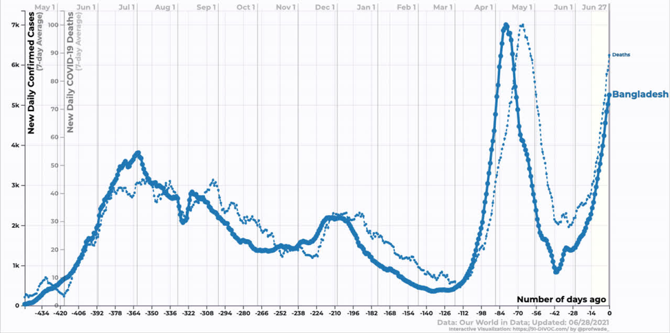
Source: https://91-divoc.com/pages/covid-visualization/

Moving onto developed counties, the UK has seen an explosion of cases corresponding to the introduction and growth of Delta. The interesting thing here is that while deaths have increased, they have increased by far less than one might expect looking at the last wave. Similarly, hospitalizations have increased, but not by that much. Why? One word: Vaccines.

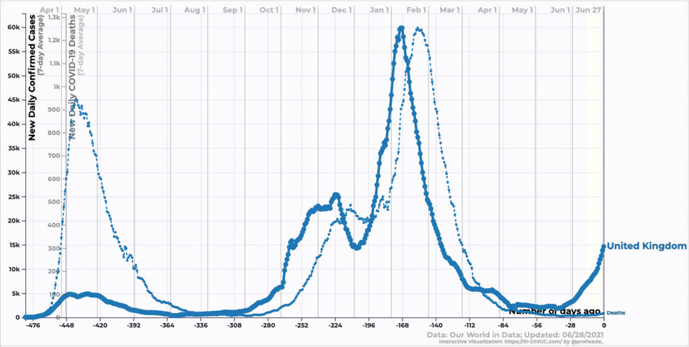
Source: https://91-divoc.com/pages/covid-visualization/

The vaccine rollout in the UK, as in the US, focused heavily on older age groups providing them with some protection against infection. As a result, the new infections are heavily weighted towards younger age groups that are less likely to be hospitalized and/or die.

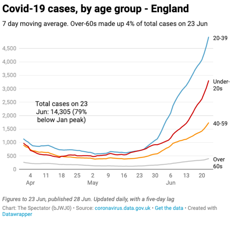
Source: The Spectator with data from the UK government

In the US, we are just starting to see the effect of the Delta variant. Reductions in case and death counts have stalled somewhat. We are still averaging ~300 deaths per day, which annualizes to ~100k dead per year. In my opinion, this remains an unacceptable death burden.

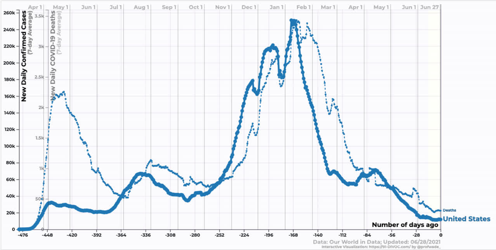
Source: https://91-divoc.com/pages/covid-visualization/

The big question is where we are going to go from here? Delta becoming the dominant strain seems highly likely over the next month or so, but what effect will that have on US case/death counts? Will we follow the UK path?

Vaccines

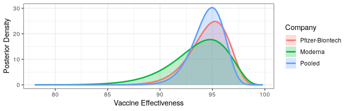
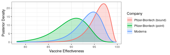
Modern science has really come through with amazingly effective vaccines. The Pfizer and Moderna vaccines showed ~95% protection against the original strain. The AstraZeneca vaccine was~70% effective (though this was later revised to 76%).

The good news is that both Pfizer and AstraZeneca appear to remain effective against the Delta variant. Based on observational data, it has been estimated that Pfizer is 88% efficacious and AstraZeneca is 60% efficacious in preventing symptomatic disease. In preventing hospitalization, they are better, with sitting at about 96% and 92% efficacy respectively. While Moderna has not been studied, I would expect it to perform similarly to Pfizer based on how highly related the methodologies are.

The bad news is that these drop offs in efficacy amount to about a doubling of the number of breakthrough infections compared to the original variant. Also, the efficacy of a single dose is just ~33%, which is too low to provide much comfort. Thus, it is critical that follow-up shots are carried out. It also means that ramping up vaccination will take some time to show effectiveness since reasonable levels of efficacy may only be achieved two weeks after the second dose.

It is unclear how other vaccines perform against Delta. Of particular interest is the effectiveness of Sinovac and Sinopharm as these are being widely deployed in China. Given their rather lackluster performance against the other strains, I am worried but keeping my fingers crossed for them.

Base Case Disease Trajectory

Based on the currently available information, the most likely scenario is that the Delta variant continues to spread across the globe outcompeting other variants. Wealthy counties with higher vaccination rates will potentially see increasing case counts similar to the UK with less severe increases in hospitalization and death. While the US has slightly lower vaccination rates compared to the UK, it has used more mRNA efficacious vaccines, which provide superior protection against community spread. This mix of superior vaccines means that the US could have less of a case count increase compared to the UK.

With increasing case counts, vaccination uptake will likely improve. However, due to the one month lag time between first dose and robust protection, it may take some time before this change in behavior is reflected in the case count curves.

With rich countries vaccinating, it seems unlikely that a large proportion of people in developing nations will have access to vaccines for some time. While the demographic bias of these countries toward the young will blunt some of the impact, a similar scenario to what played out in India could become widespread.

The impact on China is uncertain and may chart a completely different trajectory. Vaccinations in their huge population are proceeding rapidly, but the effectiveness of the vaccines they are using against Delta is an unknown. The (somewhat draconian) public health mitigation measures they have put in place have done an exceedingly good job of curbing infection. It is unknown whether these mitigation measures will hold fast against a doubling of the reproductive rate.

Big Downside Risk

Every time an infected individual comes into contact with a person resistant to infection there is an evolutionary selection pressure to overcome that resistance. For most of the pandemic the resistance has stemmed from previous SARS-CoV-2 infection. Only recently have we had significant population percentages with vaccine-initiated resistance.

The base case scenario, where there are many infected people engaging in transmission in a population with many vaccinated individuals, is a dangerous mix that could potentially lead to a vaccine resistant variant. A variant that could bypass the protections afforded by vaccination would be a radically negative outcome both from a humanitarian and economic perspective.

Economic Impacts

Many people cite the lockdowns as the cause of all of the economic woes in the age of Covid-19. These people are wrong. Covid-19 infections, hospitalizations and deaths were the cause of the economic crisis. The lockdowns were a reflection of what most people were already doing in response to the risks that they saw. We know this because states with lockdowns experienced similar drops in mobility (a proxy for economic activity at the time) as those who had not yet implemented them.

The reason the economy is reopening is because the risk has decreased and people are acting accordingly. If risk increases people will respond to that risk by protecting themselves. At previous points in the pandemic this meant social distancing, reducing indoor activities, etc. These risk mitigation behaviors had severe economic consequences, especially for the services sector.

If deaths and hospitalizations do not rise dramatically, individuals may not see the need to engage in any risk mitigation. If they do engage in risk mitigation, unvaccinated US residents have the luxury of our large supply of vaccine and may choose vaccination as their mitigation behavior. Vaccination is free, easy and has little in the way of economic consequences.

Most emerging market countries have little protecting them from similar economic consequences to those experienced by India. The effect on China, the world’s second largest economy, is uncertain because the effect of Delta on that country is similarly uncertain.

Final thoughts

The Delta variant is roughly twice as infectious as “regular” SARS-CoV-2 (Covid-19), which is roughly twice as infectious as influenza. This huge increase has significant humanitarian and economic consequences for the world.

Vaccines have been unevenly distributed around the world, with developed countries taking the vast majority of the available doses. Looking at India and Bangladesh we can see that the spread of Delta to an unvaccinated population can lead to exponential growth in both cases and deaths. The UK, which has had one of the most successful vaccination programs in the world, was also hit by the Delta variant. Because of vaccination, these cases were concentrated in younger low-risk individuals and consequently the increase in death counts has been more modest.

Case counts in China remain negligible. The mitigation measures in place have been very successful at preventing other variants spreading in the country, but those variants are less infective than Delta. The Sinopharm and Sinovac vaccines are moderately effective, and have unknown efficacy against Delta.

I’ve tried to outline what I consider to be the most likely scenario, which is:

1. Increasing case counts in developed countries with less severe increases in death counts.
2. Increasing case and death counts in countries without access to vaccines.
3. Uncertain trajectory for China.

This scenario is predicated on the data that we currently have available. Estimates of reproductive rate and vaccine effectiveness using observational data are challenging and our understanding is subject to potentially strong revisions.

The best thing we can do right now is vaccinate as many people as possible. Keeping case counts low, even among young people, decreases the selective pressure that leads to new, potentially worse, variants. Sharing vaccine with less developed nations helps blunt the impact of Delta variant spread on the most vulnerable groups.

I won’t lecture you on personal choices, but now is a particularly rational time to get vaccinated. The increased reproductive rate of the variant means there is a pretty good chance you’ll get infected if you are not vaccinated; maybe not in the next month, but the odds are good over a 5-year time horizon (unless you are a hermit). Given that vaccination is free, easy, and a whole lot nicer than even a mild case of Covid-19, getting vaccinated is a great way to hedge against a negative outcome that is probably pretty likely.

Okay, last one I swear. We just got updated results from the Pfizer-Biontech vaccine candidate. With 8 out of 170 cases belonging to the treatment group, the point estimate is remarkably similar to the Moderna preliminary results (~95% effectiveness). I will note that I was right in saying that the Pfizer-Biontech vaccine is likely much more effective than the 90% bound originally reported. Given that these are both very similar mRNA vaccines, the similarity in efficacy shouldn’t be radically surprising. Below is an updated plot of the posterior distribution for vaccine efficacy. I’ve added a “pooled” posterior, which assumes that the true efficacy is the same for both vaccines.

# reference: https://pfe-pfizercom-d8-prod.s3.amazonaws.com/2020-09/C4591001_Clinical_Protocol.pdf

# prior interval (matches prior interval on page 103)
qbeta(c(.025,.975),.700102,1)


# posterior pfizer
cases_treatment <- 8
cases_control <- 170 - cases_treatment
theta_ci <- qbeta(c(.025,.975),cases_treatment+.700102,cases_control+1)
rate_ratio_ci <- theta_ci / (1-theta_ci)

# effectiveness
100 * (1 - rate_ratio_ci)

xx <- (1:90)/500
yy <- sapply(xx, function(x) dbeta(x,cases_treatment+.700102,cases_control+1))
xx <- 100 * (1 - xx / (1 - xx))
ggplot() + 
  geom_area(aes(x=xx,y=yy)) + 
  theme_bw() + 
  xlab("Vaccine Effectiveness") + 
  ylab("Posterior Density")

# posterior combined
cases_treatment <- 8 + 5
cases_control <- 170 + 95 - cases_treatment
theta_ci <- qbeta(c(.025,.975),cases_treatment+.700102,cases_control+1)
rate_ratio_ci <- theta_ci / (1-theta_ci)

# effectiveness
100 * (1 - rate_ratio_ci)

xx1 <- (1:90)/500
yy1 <- sapply(xx1, function(x) dbeta(x,cases_treatment+.700102,cases_control+1))
xx1 <- 100 * (1 - xx1 / (1 - xx1))
ggplot() + 
  geom_area(aes(x=xx1,y=yy1)) + 
  theme_bw() + 
  xlab("Vaccine Effectiveness") + 
  ylab("Posterior Density")



# posterior moderna
cases_treatment <- 5
cases_control <- 95 - cases_treatment
theta_ci <- qbeta(c(.025,.975),cases_treatment+.700102,cases_control+1)
rate_ratio_ci <- theta_ci / (1-theta_ci)

# effectiveness
100 * (1 - rate_ratio_ci)



xx2 <- (1:90)/500
yy2 <- sapply(xx2, function(x) dbeta(x,cases_treatment+.700102,cases_control+1))
xx2 <- 100 * (1 - xx2 / (1 - xx2))
ggplot() + 
  geom_area(aes(x=xx2,y=yy2)) + 
  theme_bw() + 
  xlab("Vaccine Effectiveness") + 
  ylab("Posterior Density")


df <- rbind(
  data.frame(xx=xx,yy=yy,Company="Pfizer-Biontech"),
  data.frame(xx=xx2,yy=yy2,Company="Moderna"),
  data.frame(xx=xx1,yy=yy1,Company="Pooled")
)
ggplot(df) + 
  geom_area(aes(x=xx,y=yy,fill=Company),alpha=.25,position = "identity") + 
  geom_line(aes(x=xx,y=yy,color=Company),size=1) + 
  theme_bw() + 
  xlab("Vaccine Effectiveness") + 
  ylab("Posterior Density")

Both provide excellent protection. Really the only new information is that there is no meaningful difference in efficacy between the two, and hence no reason to prefer one over the other.

Some safety data was also reported:

A review of unblinded reactogenicity data from the final analysis which consisted of a randomized subset of at least 8,000 participants 18 years and older in the phase 2/3 study demonstrates that the vaccine was well tolerated, with most solicited adverse events resolving shortly after vaccination. The only Grade 3 (severe) solicited adverse events greater than or equal to 2% in frequency after the first or second dose was fatigue at 3.8% and headache at 2.0% following dose 2.

This is really good, and maybe even a bit better than Moderna's reported profile. I honestly don't know how to square this with higher averse event rates in the phase II study, where a significant number of participants had fevers after the second dose.

There were 10 severe cases of which 1 was in the treatment arm. Pooling the data from the Moderna and Pfizer studies, 7.1% of cases were severe in the treated arm versus 8.9% in the control. This difference is nowhere near significance though. So no real evidence yet that mRNA vaccines make illness milder should you be infected.

One thing that may have gone under the radar is this quote:

“We are grateful that the first global trial to reach the final efficacy analysis mark indicates that a high rate of protection against COVID-19 can be achieved very fast after the first 30 µg dose, underscoring the power of BNT162 in providing early protection,” said Ugur Sahin, M.D., CEO and Co-founder of BioNTech.

It appears that protection ramps up after the first shot, which is critical since we are in the midst of a huge surge in cases. We need immediate protection as soon as possible to reduce the death and reproductive rates.

This is a public notice that Fellows Statistics is launching a service to provide HIV/AIDS testing sites with better access to their data and statistical products based on their data.