A new version of the OpenStreetMap package is now up on CRAN, and should propagate to all the mirrors in the next few days. The primary purpose of the package is to provide high resolution map/satellite imagery for use in your R plots. The package supports base graphics and ggplot2, as well as transformations between spatial coordinate systems.
The bigest change in the new version is the addition of dozens of tile servers, giving the user the option of many different map looks, including those from Bing, MapQuest and Apple.
You can also render maps from cloudmade.com which hosts tons of map tilings. Simply set the “type” parameter to “cloudmade-<id>” where <id> is the cloudmade identifier for the map you want to use. Here is a sample:
Maps are initially put in a sperical mercator projection which is the standard for most (all?) map tiling systems, but can easily be translated to long-lat (or any other projection) using the openproj function. Maps can be plotted in ggplot2 using the autoplot function.
mapLatLon = openproj(map)
autoplot(mapLatLon)
The package also has a Java GUI to help with map type selection, and specification of coordinates to bound your map. clicking on the map will give you the latitude and longitude of the point clicked.
launchMapHelper()
Probably the main alternative to OpenStreetMap is the ggmap package. ggmap is an excellent package, and it is somewhat unfortunate that there is a significant duplication of effort between it and OpenStreetMap. That said, there are some differences that may help you decide which to use:
Reasons to favor OpenStreetMap:
More maps: OpenStreetMap supports more map types.
Better image resolution: ggmap only fetches one png from the server, and thus is limited to the resolution of that png, whereas OpenStreetMap can download many map tiles and stich them together to get an arbitrarily high image resolution.
Transformations: OpenStreetMap can be used with any map coordinate system, whereas ggmap is limited to long-lat.
Base graphics: Both packages support ggplot2, but OpenStreetMap also supports base graphics.
Reasons to favor ggmap:
No Java dependency: ggmap does not require Java to be installed.
Geocoding: ggmap has functions to do reverse geo coding.
Google maps: While OpenStreetMap has more map types, it currently does not support google maps.
This is a quick note on profiling your compiled code on the mac. It is important not to guess when figuring out where the bottlenecks in your code are, and for this reason, the R manual has several suggestions on how to profile compiled code running within R. All of the methods are platform dependent, with linux requiring command line tools (sprof, and oprofile). On the mac there are some convenient GUI tools built in to help you out.
Our test code is drawn from the ergm package, and fits a network model to a small graph. This model is fit using markov chain monte carlo, so we expect most of the time to be spent drawing MCMC samples.
The quickest way to get an idea of where your program is spending time is to open Activity Monitor.app and select the R process while the above code is running. Then click sample, which should result in something like:
In order to get down to the interesting code, you’ll have to wade though a bunch of recursive Rf_eval and do_begin calls used by R. Finally though we see the MCMCSample function in ergm.so which contains almost all of the samples. So it is as we expected, the MCMC sampling takes up all the time. Underneeth that we see calls to:
ChangeStats: calculates the network statistics
MH_TNT: calculates the metropolis proposal
ToggleEdge: alters the network to add (or remove) an edge
But how much these contribute is a bit difficult to see here. Enter the Time Profiler in Instruments.app. You can launch this program from within Xcode.app under Xcode – Open Developer Tool – Instruments. Once Instruments is open, click Library and drag the Time Profiler into the program. Then, while the R code is running, select ‘Attach to Process’ – R and click record. You should get something like: Like in the Activity Monitor, we have to drill down past all of the recursive Rf_eval calls, but once we do, we see that ChangeStats is taking 44.6% of the time, MH_TNT takes 30.9% and ToggleEdges takes 11.7%. We could further expand these out to identify possible targets for optimization within each of these functions.
So there you have it. Apple makes it really easy to profile your compiled code. One issue that I ran into is to make sure that your Xcode is up-to-date and that Instruments is version 4.0 or above. I experienced some crashes profiling R with older versions.
This is a really great exposition on an
infographic. Note that the design elements and “chart junk” serve
to better connect and communicate the data to the viewer. The
choice not to go with pie charts for the first set of plots is a
good one. The drawbacks of polar representations of proportions is
very well know to statisticians, but designers often feel that
circular elements are more pleasing in their infographics. This
bias toward circular representations is sometimes justifiable.
After all, if your graphic is pretty then no one will take the time
to look at it.
I’m usually quite a big fan of the content syndicated on R-Bloggers (as this post is), but I came across a post yesterday that was as statistically misguided as it was provocative. In this post, entitled “The Surprisingly Weak Case for Global Warming,” the author (Matt Asher) claims that the trend toward hotter average global temperatures over the last 130 years is not distinguishable from statistical noise. He goes on to conclude that “there is no reason to doubt our default explaination of GW2 (Global Warming) – that it is the result of random, undirected changes over time.”
These are very provocative claims which are at odds with the vast majority of the extensive literature on the subject. So this extraordinary claim should have a pretty compelling analysis behind it, right?…
Unfortunately that is not the case. All of the author’s conclusions are perfectly consistant with applying an unreasonable model, inappropriate to the data. This in turn leads him to rediscover regression to the mean. Note that I am not a climatologist (neither is he), so I have little relevant to say about global warming per se, rather this post will focus on how statistical methodologies should pay careful attention to whether the data generation process assumed is a reasonable one, and how model misspecification can lead to professional embarrassment.
His Analysis
First, let’s review his methodology. He looked at the global temperature data available from NASA. It looks like this:
Average global temperatures (as deviations from the mean) with cubic regression
He then assumed that the year to year changes are independent, and simulated from that model, which yielded:
Here the blue lines are temperature difference records simulated from his model, and the red is the actual record. From this he concludes that the climate record is rather typical, and consistant with random noise.
A bit of a fly in the ointment though is that he found that his independence assumption does not hold. In fact he finds a negative correlation between one years temperature anomaly and the next:
Any statistician worth his salt (and indeed several of the commenters noted) that this looks quite similar to what you would see if there were an unaccounted for trend leading to a regression to the mean.
Bad Model -> Bad Result
The problem with using an autoregressive model here is that it is not just last year’s temperatures which determine this year’s temperatures. Rather, it would seem to me as a non-expert, that temperatures from one year are not the driving force for temperatures for the next year (as an autoregressive model assumes). Rather there are underlying planetary constants (albedo and such) that give a baseline for what the temperature should be, and there is some random variation which cause some years to be a bit hotter, and some cooler.
Remember that first plot, the one with the cubic regression line. Let’s assume that data generation process is from that regression line, with the same variance of residuals. We can then simulate from the model to create an fictitious temperature record. The advantage of doing this is that we know the process that generated this data, and know that there exists a strong underlying trend over time.
Simulated data from a linear regression model with cubic terms
If we fit a cubic regression model to the data, which is the correct model for our simulated data generation process, it shows a highly significant trend.
              Sum Sq  Df F value    Pr(>F)
poly(year, 3)  91700   3  303.35 < 2.2e-16 ***
Residuals      12797 127
We know that this p-value (essentially 0) is correct because the model is the same as the one generating the data, but if we apply Mr. Asher’s model to the data we get something very different.
Auto regressive model fit to simulated data
His model finds a non-significant p-value of .49. We can also see the regression to the mean in his model with this simulated data.
Regression to the mean in simulated data
So, despite the fact that, after you adjust for the trend line, our simulated data is generating independent draws from a normal distribution, we see a negative auto-correlation in Mr. Asher’s model due to model misspecification.
Final Thoughts
What we have shown is that the model proposed by Mr. Asher to “disprove” the theory of global warming is likely misspecified. It fails to to detect the highly significant trend that was present in our simulated data. Furthermore, if he is to call himself a statistician, he should have known exactly what was going on because regression to the mean is a fundamental 100 year old concept.
———————-
The data/code to reproduce this analysis are available here.
The 2012 election is over and in the books. A few very close races remain to be officially decided, but for the most part everything has settled down over the last week. By all accounts it was a very good night for the Democrats, with wins in the presidency, senate and state houses. They also performed better than expected in the House of Representatives. If we take the results as they stand now, the Democrats will have 202 seats v.s. the Republican’s 233 seats, a pick-up of 9 relative to the 2010 election. This got me thinking about how the Republicans could have maintained 54% of the house seats during a Democratic wave election.
Since I’m a statistician, the obvious answer was to go get the data and find out. Over the last few days, I was able to obtain unofficial vote counts for each congressional race except 3. The results from two unopposed Democrats in Massachusetts’ 1st and 2nd district, and one unopposed Republican from Kansas’ 1st district will not be available until the final canvas is done in December. Not including these districts 55,709,796 votes were cast for Democrats, v.s. 55,805,487 for Republicans, a difference of less than 100,000 votes.
Both of the candidates from Massachusetts also ran unopposed in 2008, where they garnered 234,369 and 227,619 votes respectively, which seems like a good estimate for what we can expect this year. In 2008 Kansas’ 1st district had a total of 262,027 votes cast. We will assign all of them to the Republican candidate as an (over) estimate, as the old 2002 district lines are similar to their 2012 placements. Using these numbers we get estimated vote counts of 56,171,784 for the Democrats and 56,067,514 for the Republicans, leading to a 100,000 vote advantage for the Democrats. Either way, this election was a real squeaker in terms of popular vote, which in percentage terms is 50.046% to 49.954%. Until the full official results are released, I would classify this as “too close to call,” but find a Democrat popular vote victory likely.
Nate Silver recently looked at the differences in the number of votes cast in 2008 v.s. those already reported in 2012, and found that California has reported 3.4 million fewer votes this election than 2008, suggesting that millions of mail-in ballots remain waiting to be certified. Somewhat similarly, New York reported 1.5 million fewer votes, though this may be due (at least in part) to the effects of hurricane Sandy. These were the only two states with differences > 1 million, and they both lean heavily Democratic, which may well push the popular vote totals for the Democrats into “clear winner” territory.
In a certain sense, the winner of the popular vote is irrelevant, as the only thing that matters in terms of power is the number of seats held by a party. But if the Democrats win, then they can reasonably claim that they (even as the minority party) are the ones with the mandate to enact their agenda.
Even though the popular vote is razor close in the current unofficial results, the distribution of seats is certainly not. We shouldn’t expect there to be a perfect correspondence between the popular vote and seats, because who wins the seats depends on how the population is divided up into congressional districts. As a simplified example consider three districts, each with 100,000 voters. District 1 is heavily Democratic, with 100% of votes going to the democratic candidate, while districts 2 and 3 are swing districts where 51% of the vote goes to the Republicans. In this simplified example, the Democrats would win nearly 2/3 of the popular vote, but only 1/3 of the seats.
So, if we expect there to be a discrepancy between popular vote and seat totals, the question then becomes: Is this election unusual? To answer this, we can look at the official historical record going back to 1942 which gives us the following:
Relationship between popular vote, and share of congressional seats (1942-2012)
In almost every election in the last 70 years, the party with the popular vote victory also won the majority of seats. The only exception to this was 1996, where the Democrats won the popular vote, but failed to attain a majority in congress. If 2012 turns out to be a popular vote victory for the Democrats, then their seat deficit would be unheard of in living memory. On the other hand, there was a very close election in 1950, where the Republicans lost by a margin of just 0.04%, but ended up with only 199 seats to the Democrats 234.
Redistricting, Gerrymandering, oh my!
Whether or not the official vote tally goes to the Democrats, the 2012 House of Representatives electoral landscape is unusual. The seat totals clearly favor the Republicans, but why? Some have noted that the congressional district lines were redrawn following the 2010 Census, a process that in many states is controlled by the state legislature, and that many of these lines seem to be constructed to maximize the political advantage of one party or the other. I was initially skeptical of these claims. After all, the two years most comparable to 2012 are 1996 and 1950, neither of which are particularly near a redistricting period. As is often the case, an examination of the data revealed evidence that was counter to my expectations.
First, let us explore how one would draw lines that maximize party advantage. Remember in our simple three district example, the advantage was gained by bunching all of the Democratic voters into one district, and maintaining slim advantages in the other two. So, the rule is to spread out your own vote into many districts, and consolidate your opponents voters into just a few. This can be a difficult geometric “problem” to solve, but an easy way to think about one possible route toward a solution is to focus on the swing districts. If a district is very close, you will want to alter its location so that it has just enough more Republican votes to make it a safe bet for your party. Ideally you will want to take these Republican votes from a safe Democratic district, making it even more Democratic. What you can then expect when you look at the distribution of districts is a clump of very safe Democratic districts, a clump of safe, but not overwhelmingly safe, Republican districts, and very few toss-up districts. This is what we call a bimodal distribution, and the process of redistricting with a focus on political gain is known as gerrymandering. There is nothing particularly Republican about it. Both political parties engage in gerrymandering, the difference being whether or not they control the redistricting process, and to what degree are they willing to contort the shape of their districts.
Authority to draw lines
# of Congressional districts
Democratic party
44
Republican party
174
Split between parties
83
Independent Commission
88
Only one district in the state
7
Non-partisan legislature
3
Temporary court drawn
36
The Republican party was in control of the redistricting of 174 districts, v.s. just 44 for the Democrats. Just to give a specific example, Ohio had a Republican controlled redistricting process, which though wildly successful for Republicans, lead to torturously shaped districts. Republicans won 52.5% of the vote in Ohio, but obtained a staggering 75% of the seats.
But that is just one state, what about the rest of the districts? If we plot the proportion of people in each district that go to the Democrats, broken down by who was in control of redistricting we see clear evidence of clumping into safe, but not overwhelmingly safe territory for the redistricting party.
Share of vote by who controlled redistricting
The way to read this plot is that each point represents a district, with its position being the proportion of people in the district who voted for the Democratic candidate. The lines represent a smoothed estimate of the distribution, with wider parts indicating increased density. Among the districts where Republicans had control, we see a characteristic bimodal distribution, with many districts chosen to be relatively safe Republican strongholds, with a smaller group of heavily Democratic districts. The same trend may be present in the Democratically controlled districts, but there are too few of them to see the trend clearly. Alternatively, in districts where the decision making is split between parties, or delegated to an independent group, we see a more natural distribution of vote shares, with a good number of toss-up districts.
But can we prove that it swung the election?
To parse out the effect of redistricting on the election results in a non-descriptive sense, it is necessary to construct (a simple idealized) model of how redistricting affects the probability of winning a district. To do this, we assume that the probability of winning a district within a state is related to the partisanship of the state (i.e. we expect a higher proportion of Republican seats in Alabama as compared to New York), which we will measure by the share of the vote that Romney won in the state. Second, control of redistricting (either Democratic, Republican, or Independent/Split) yields an increase (or decrease) in the odds of a win. We slap these two together into a standard statistical model known as a logistic regression, which yields the following:
Variable
Df
Chi-squared
p-value
Romney vote
1
31.4
<0.001
Redistricting control
2
9.1
0.010
Residuals
385
This table tells us two important things through its p-values. With p-values, the closer to 0, the more significant the relationship. First, that the partisanship of a district matters, because the proportion voting for Romney is very significantly related to the probability of congressional control. Secondly, control of redistricting matters. If the redistricting process were fair, we would see the magnitude of the trends that we see in this data only once every thousand years (10 years between redistricting / 0.010 ). This gives us a high degree of confidence that political concerns are the driving force in redistricting when politicians are put in charge of it (shocking, I know).
This effect is relatively large. Consider an idealized swing state, where Romney won exactly 50% of the vote. Our model estimates the proportion of the congressional delegation who are Democrats as:
Estimates of the average proportion of a congressional delegation from a true swing state who are Democrats based on a logistic regression
Here the model estimates that districts from an independent/split source are roughly unbiased with an estimated proportion of seats of 48%. If the Republicans control the process then we would expect only 31% of the delegation to be Democrats. This is slightly above what we observed in Ohio, where only 25% of the delegation were Democrats, despite Romney’s percentage of the vote being nearly 50%. With the Democrats in control we see a smaller bias than the Republicans with an estimated 56% belonging to the Democratic party, but our confidence in this estimate (denoted by the red dotted lines) is small due to the small number of redistricting opportunities that they had.
A perfect world
What would have happened if the entire redistricting process was controlled by independent or bipartisan agreement? Well, our simple model can tell us something about that. By counterfactually assuming that all redistricting was done independently or by split legislature, it estimates that the proportion of Democrats in the current congress would be, on average, 52%. If Democrats got to pick all the lines it would be 59%, and under complete Republican control it would be just 37%.
Conclusions
So what lessons can we take away from this analysis? Control of the redistricting process is a powerful tool for those who would use it as a tool. The model estimates that who controls the process could yield 17% point swings (56%-39%) in a typical swing state. This is consistent both with the results from the general election as a whole, and Ohio in particular. While I would love to see the implementation of an algorithmic solution to the problem of district formation (if only to hear the pundits trying to say minimum isoperimetric quotient), it appears that independent commissions, or even bipartisan agreement within a legislative body are sufficient to have fair lines. As of now, 6 states decide their districts based on an independent commission, and it is hard to think of an honest argument why every state should not adopt this model. Economics teaches us that incentives matter, and if you give politicians the incentive to bias districts in their favor, it is a safe bet that they will do so.
————————————–
Fellows Statistics provides experienced, professional statistical advice and analysis for the corporate and academic worlds.
An update to the wordcloud package (2.2) has been released to CRAN. It includes a number of improvements to the basic wordcloud. Notably that you may now pass it text and Corpus objects directly. as in:
wordcloud("May our children and our children's children to a
thousand generations, continue to enjoy the benefits conferred
upon us by a united country, and have cause yet to rejoice under
those glorious institutions bequeathed us by Washington and his
compeers.",colors=brewer.pal(6,"Dark2"),random.order=FALSE)
This bigest improvement in this version though is a way to make your text plots more readable. A very common type of plot is a scatterplot, where instead of plotting points, case labels are plotted. This is accomplished with the text function in base R. Here is a simple artificial example:
Notice how many of the state names are unreadable due to overplotting, giving the scatter plot a cloudy appearance. The textplot function in wordcloud lets us plot the text without any of the words overlapping.
textplot(loc[,1],loc[,2],states)
A big improvement! The only thing still hurting the plot is the fact that some of the states are only partially visible in the plot. This can be fixed by setting x and y limits, whch will cause the layout algorithm to stay in bounds.
Another great thing with this release is that the layout algorithm has been exposed so you can create your own beautiful custom plots. Just pass your desired coordinates (and word sizes) to wordlayout, and it will return bounding boxes close to the originals, but with no overlapping.
okay, so this one wasn’t very creative, but it begs for some further thought. Now we have word clouds where not only the size can mean something, but also the x/y position (roughly) and color. Done right, this could add whole new layer of statistical richness to the visually pleasing but statistically shallow standard wordcloud.
The book R for Dummies was released recently, and was just reviewed by Dirk Eddelbuettel in the Journal of Statistical Software.
Dirk is an R luminary, creating such fantastic works as Rcpp. R for Dummies seems to have beaten Dirk’s natural disinclination to like anything with “for Dummies” appended to it, receiving a pretty positive review. Here is the last bit:
“R for Dummies may well break new ground, and introduce R to new audiences. The pricing is aggressive and should help the book to find its way into the hands of a large number of students, data analysis practitioners as well as researchers. They will find a well-written and easy-to-read introduction to the language and environment – if they can overcome any initial bias against a Dummies title as this reviewer did.”
I haven’t had a chance to read the text, but I have worked (albeit briefly) with Andie de Vries who is one of the authors. He is the author of several R packages up on CRAN, is a regular contributor to the R tag on Stack Overflow, and has a nuanced understanding of the language.
It is difficult for R package authors to know how much (if at all) their packages are being used. CRAN does not calculate or make public download statistics (though this might change in the relatively near future), so authors can’t tell if 10 or 10,000 people are using their work.
Deducer is in much the same boat. We can’t know how many people are downloading it, but we can get an idea of its usage by looking at how many people are accessing the online manual. The site recently passed the quarter of a million page view milestone, with close to 75k visits.
Deducer.org is now consistently getting over 3,000 page views a week, which is about 4-5 times greater than the same time 2 years ago. Traffic growth seems pretty consistant and surprisingly linear, indicating that we have a solid user base and adoption is progressing at a good rate. Exactly what the size of that user base is and the rate of adoption is something that can’t really be answered with raw traffic data, but the trends look unequivocally good.
With the addition of add-on packages like DeducerSpatial and DeducerPlugInScaling created by myself and a budding community of developers, I am very optimistic about the outlook for continued growth. If you have not given Deducer a try, either for personal use or in the classroom, now is a great time to start.
————————————–
Fellows Statistics provides experienced, professional statistical advice and analysis for the corporate and academic worlds.
I’ve been doing R/Java development for some time, creating packages both large and small with this tool chain. I have used Eclipse as my package development environment almost exclusively, but I didn’t realize how much I relied on the IDE before I had to do some serious R/C++ package development. My first Rcpp package (wordcloud) only used a little bit of complied code, so just using a standard text editor was enough to get the job done, however when I went on to a more complex project, TextWrangler just wasn’t cutting it anymore. Where was my code completion? Where were my automatically detected syntax errors?
I found myself spending more time looking up class APIs, fixing stupid errors, and waiting for R CMD INSTALL to finish than I did coding. Unfortunately the internet did not come to the rescue. I searched and searched but couldn’t find anyone who used a modern IDE for package development with compiled code. In particular I wanted the following features.
Code completion. What methods does that class have again? What arguments does that function take? Perhaps everyone is just smarter than me, but I can’t seem to keep the whole R/Rcpp API in my head. I just want to hit ctrl+space and see what my options are:
Syntax error detection. Oh, I meant hasAttribute. Whoops, forgot that semicolon again.
Incremental builds. It takes a long time for R CMD INSTALL to complete. The package that I am currently working on takes 2 minutes and 30 seconds to install. I don’t want to have to wait for a full install every time I make a small change to a function I am playing with.
R and C++ syntax highlighting. Editing good looking code makes for a better coding experience.
The solution I found is a combination of Eclipse, Rcpp and RInside. Rcpp is undeniably the best way to embed high performance C++ code within R. It makes writing C++ code with native R objects a breeze. Even John Chambers is unhappy with the lack of elegance in the R/C interface. Rcpp uses some of the more advanced language features in C++ to abstract away all of the ugliness. RInside on the other hand embeds R within a C++ program.
The steps below will show you how to link up Eclipse with Rcpp to get code completion and syntax error detection, then RInside will be used to link up R with Eclipses build and run systems allowing for incremental building and rapid prototyping.
Step 1: Download Eclipse
You will need to download the CDT version of eclipse for c/c++ development. It can be obtained at http://www.eclipse.org/cdt/.
Step 2: Install statet
statet is an eclipse plug-in supporting R integration. Follow the installation instructions at http://www.walware.de/goto/statet. R will need to be configured, which is covered in section 3 of Longhow Lam’s user guide.
In the file system navigate to your R working directory. There you should find a new folder labeled MyCppPackage. Drag the contents of that folder into your project in eclipse.
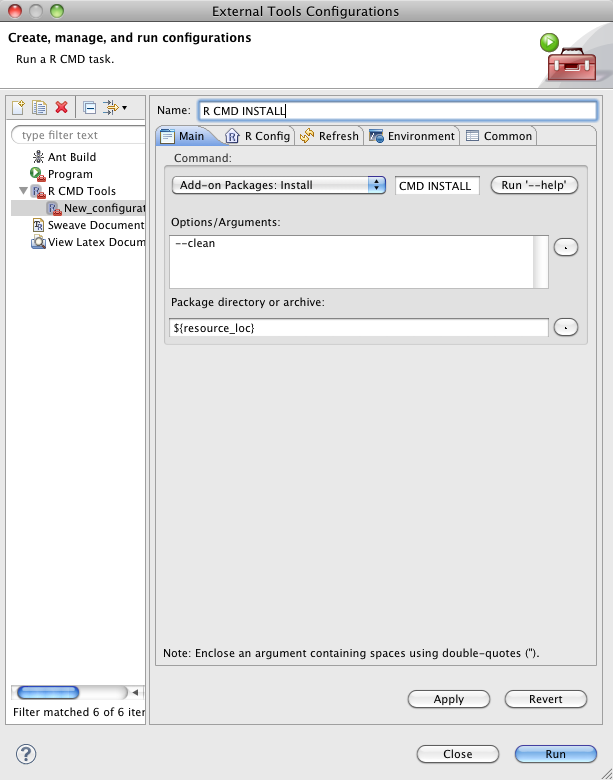
Step 5: Making the package installable
Open the external tools configurations and create a new statet R CMD Tools configuration for R CMD INSTALL. Change the directory from resource_loc to project_loc. Note, you will probably want to also add the command line argument “–clean” so that temporary files created during the install process are removed. If you want the fastest possible installation, use “–no-test-load –no-multiarch –clean”.
Your shiny new Rcpp project should now be installable with the click of a button. Run the configuration (you should an install log in the console) and check that the package is now loadable by running library(MyRcppPackage) in R.
Step 6: Setting up links and properties
Now eclipse knows how to install the package, but it doesn’t know what any of the symbols in your C++ files mean because it can’t see the Rcpp package. If you look at the rcpp_hello_world.cpp file you should see a bunch of bugs.
In this step we will set up the project properties necessary for Eclipse to link up with R, Rcpp and RInside. There may be a few things that you need to change for your system. Notably, the directories listed below all start with /Library/Frameworks/R.framework/Resources. This is the default R_HOME for Mac OS X. If your R home is located in a different place, or you have a user library directory where Rcpp and RInside are installed, you will need to edit the directories accordingly. Also, the architecture for my R is x86_64, so if your architecture is different, you will need to change this.
Right click on MyCppPackage and select properties.
Add references to the header files for R, Rcpp and RInside to the G++ compiler includes.
/Library/Frameworks/R.framework/Resources/include
/Library/Frameworks/R.framework/Resources/library/Rcpp/include
/Library/Frameworks/R.framework/Resources/library/RInside/include
(note: these may be different on your system depending on your R_HOME and library paths)
(edit: I’ve removed the include directive for the /Rcpp/include/Rcpp directory as it is not needed and can lead to conflicting references for string.h on case-insensitive operating systems).
Add a reference to the R library to G++ linker – Libraries.
(edit: I’ve removed the reference to Rcpp/lib/x86_64/libRcpp.a as Rcpp is header only (as of 0.11.0))
Add the “-arch x86_64” architecture flag for g++ compiler. This option is found in the Miscellaneous settings. If your computer’s architecture is different, set the flag accordingly.
Set the g++ Compiler – Preprocessor symbol INSIDE. This is used in the main.cpp file in the next section.
Step 7: Enabling building and launching
Create a new c++ file main.cpp in the src folder with the following code
#ifdef INSIDE
#include <Rcpp.h>
#include <RInside.h>                    // for the embedded R via RInside
#include "rcpp_hello_world.h"
using namespace Rcpp;
using namespace std;
int main(int argc, char *argv[]) {
    RInside R(argc, argv);              // create an embedded R instance
    SEXP s = rcpp_hello_world();
    Language call("print",s);
    call.eval();
    return 0;
}
#endif
Execute Project – “Build All”. You should see the project building in the eclipse console, ending with **** Build Finished ****.
Next, go to Run – “Run Configurations”.
Create a new C++ run configuration set to launch the binary Debug/MyCppPackage
Hit run. You should then see the binary building and running. The output of main.cpp will be emitted into the Eclipse console. This allows you to do rapid prototyping of c++ functions even if they require the full functionality of R/Rcpp.
You can also make use of Eclipse’s extensive and very useful code sense to both detect errors in your code, and to assist in finding functions and methods. ctrl+space will trigger code completion
Final thoughts
Rcpp has made R package development with C++ code orders of magnitude easier than earlier APIs. However, without the features modern IDE, the developers life is made much harder. Perhaps all the old school kids with Emacs/ESS have trained their brains to not need the features I outlined above, but I am certainly not that cool. I found that I was at least 4-5 times more productive with the full Eclipse set-up as I was prior.
After following the steps above, you should have a template project all set up with Eclipse and are ready build it out into your own custom Rcpp based package. These steps are based on what worked for me, so your milage may vary. If you have experiences, tips, suggestions or corrections, please feel free to post them in the comments. I will update the post with any relevant changes that come up.
 You can also render maps from cloudmade.com which hosts tons of map tilings. Simply set the “type” parameter to “cloudmade-<id>” where <id> is the cloudmade identifier for the map you want to use. Here is a sample:
 Maps are initially put in a sperical mercator projection which is the standard for most (all?) map tiling systems, but can easily be translated to long-lat (or any other projection) using the openproj function. Maps can be plotted in ggplot2 using the autoplot function.
 The package also has a Java GUI to help with map type selection, and specification of coordinates to bound your map. clicking on the map will give you the latitude and longitude of the point clicked.


