Last week a question came up on Stack Overflow about determining whether a variable is distributed normally. Some of the answers reminded me of a common and pervasive misconception about how to apply tests against normality. I felt the topic was general enough to reproduce my comments here (with minor edits).
Misconception: If your statistical analysis requires normality, it is a good idea to use a preliminary hypothesis test to screen for departures from normality.
Shapiro’s test, Anderson Darling, and others are null hypothesis tests against the the assumption of normality. These should not be used to determine whether to use normal theory statistical procedures. In fact they are of virtually no value to the data analyst. Under what conditions are we interested in rejecting the null hypothesis that the data are normally distributed? I, personally, have never come across a situation where a normal test is the right thing to do. The problem is that when the sample size is small, even big departures from normality are not detected, and when your sample size is large, even the smallest deviation from normality will lead to a rejected null.
Let’s look at a small sample example:
> set.seed(100)
> x <- rbinom(15,5,.6)
> shapiro.test(x)

Shapiro-Wilk normality test

data: x
W = 0.8816, p-value = 0.0502

> x <- rlnorm(20,0,.4)
> shapiro.test(x)

Shapiro-Wilk normality test

data: x
W = 0.9405, p-value = 0.2453
In both these cases (binomial and lognormal variates) the p-value is > 0.05 causing a failure to reject the null (that the data are normal). Does this mean we are to conclude that the data are normal? (hint: the answer is no). Failure to reject is not the same thing as accepting. This is hypothesis testing 101.
But what about larger sample sizes? Let’s take the case where there the distribution is very nearly normal.
> library(nortest)
> x <- rt(500000,200)
> ad.test(x)

Anderson-Darling normality test

data: x
A = 1.1003, p-value = 0.006975

> qqnorm(x)
> hist(x,breaks=100)
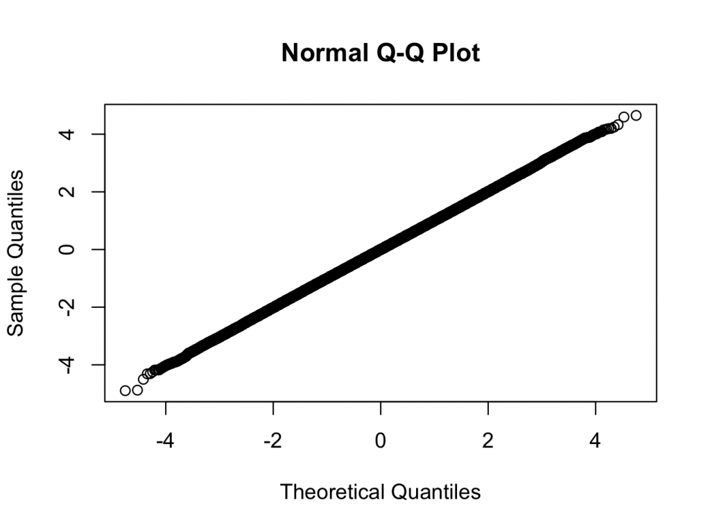
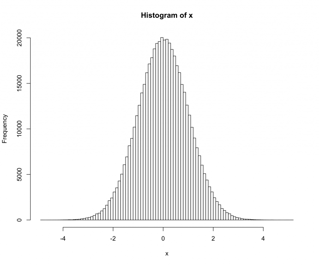
Here we are using a t-distribution with 200 degrees of freedom. The qq and histogram plots show the distribution is closer to normal than any distribution you are likely to see in the real world, but the test rejects normality with a very high degree of confidence.
Does the significant test against normality mean that we should not use normal theory statistics in this case? (Another hint: the answer is no 🙂 )


5 replies on “Normality tests don’t do what you think they do”
[…] Normality tests don’t do what you think they do « Fells Stats […]
[…] Normality tests don’t do what you think they do « Fells Stats […]
I normally (pun intended) worry much more about independence and heterocedasticity (in that order). I start thinking about normality when dealing with clear deviations (binary responses, counts, etc).
I do agree with Luis, homocedasticity or heterocedasticity is more important. Both normality and homogeneity of the variance are require to perform many test including ANOVA (pretty robust to deviation from normaliy but sensitive to non homogenous variance).
An other point is that you are comparing two different tests the shapiro.test and the ad.test, mainly because I suppose by using 500000 you could not use shapiro which is limited to 5000 value, however if you use the shipiro test but limit your sample size to 5000
> x shapiro.test(x)
HO is not rejected
W = 0.9997, p-value = 0.8337
I usually use both shapiro.test (Normality) and bartlett.test (Homocedasticity) and then I am able to decide whether I use an ANOVA or Kruskal_test.
I do not know much about the ad.test so I cannot comment on it.
The point is still valid for shapiro.test at sample sizes of 5000. For example if we look at a t-distribution with df=100 (which is still very near normal):
> set.seed(100)
> x <- rt(5000,100) > shapiro.test(x)
Shapiro-Wilk normality test
data: x
W = 0.9993, p-value = 0.04019
I disagree with your use of shapiro.test and bartlett.test to decide what statistical procedure to use. Both of these are tests _against_ the assumption in question, thus you will end up always thinking you are okay at small sample sizes and always using robust methods at large sample sizes.
Instead look at the histograms and qq-plots instead of calculating shapiro.test, and look at the sample variances instead of using bartletts.test. If you are worried by what you see, run some simulations of the procedure under the null hypothesis with the observed variances and see if the p-value distribution is sufficiently close to uniform.